In the previous article, we learned about the importance of volatility and predicted it in finance. In this article, we will learn in detail the volatility forecasting methods, from traditional statistical models to machine learning and deep learning models, which are growing in the current artificial intelligence.

Traditional Statistical Methods in Crypto Volatility Forecasting

Traditional statistical models—like GARCH, ARIMA and EWMA—were the earliest tools for forecasting volatility in crypto markets (e.g. Bitcoin, Ethereum) by mining historical price data, on-chain metrics and order-book depth. They combine past returns, realized volatility and mathematically rigorous formulas to estimate future swings. Their advantages include:

• Simplicity & speed: fast backtests and deployment on spot and derivatives (futures/options) data
  
• Theoretical rigor: well-studied properties in traditional finance

However, they often struggle during:

• Black-swan moves (e.g. DeFi protocol exploits, exchange hacks)
  
• Nonlinear contagion between altcoins and stablecoins
  
• Whale activity & funding-rate spikes in perpetual futures
  
• On-chain network effects (e.g. sudden NFT mint rushes or liquidity-pool drains)

In those cases, hybrid approaches that layer in implied volatility from crypto options markets, sentiment analysis (social volume, Google Trends), or machine-learning on-chain indicators can help capture the complex dynamics that pure statistical models miss.

1. Rolling Variance

Rolling Variance is one of the simplest methods to estimate the volatility. This method uses the sliding average of the variance (or standard deviation) from the property yield chain in a fixed time window to forecast the current volatility or the near future. With intuitive and easy to implement, the Rolling Variance is often used as a preliminary tool to assess the level of market fluctuations.

Advantage:

– Simple and intuitive: This method is easy to calculate, understand and does not require intensive knowledge about statistics.

– Quick: Provide instant estimates of the level of fluctuations based on the nearest historical data.

– Suitable for limited data: Do not require large amounts of data, suitable for small markets or new assets.

Limits:

– Slow reaction: This method assigns uniform weight to all observations in the window, leading to slow response to market shocks or sudden changes.

– Simplifying assumption: Volatility assumption is the constant in the time window that does not reflect the Time-Varying nature of the volatility.

– Sensitive to time windows: The result depends on the length of the N window, and the selection of N is often subjective, lacking a clear theoretical basis.

– Do not grasp the fluctuating cluster: Sliding variance cannot describe the phenomenon of “volatility clustering” – an important feature of the financial chain, where high fluctuations are often followed by similar stages.

2. ARCH model (Auto Regressive Conditional Heteroskedasticity)

The ARCH model, introduced by Robert Engle in 1982, marked a turning point in modeling of financial volatility. As a pioneering model in the officialization of the concept of conditional variance, the ARCH assumes that the volatility at the present time depends on the square of the square of the shocks (errors) in the past. This work has brought the Economic Nobel Prize, affirming the importance of the model in finance.

Advantage:

– Fluctuing cluster model: ARCH is the first model to capture the phenomenon of “Volatility Cluster” – high fluctuations often go together.

– Contact the shock: Volatility depends on the magnitude of the past shocks, increasing practicality. Certain theoretical basis: is the foundation for many modern fluctuations.

Limits:

– High level requirements: usually need large levels, leading to many parameters and risks of violating model conditions.

– Symmetrical effects: Not reflecting “leverage effects”, when bad news often increases the volatility stronger than good news.

– Limitations: Lack of flexibility when faced with sudden structural changes.

3. Garch model (Generalized Arch)

Developed by Bollerslev’s heart in 1986, the Garch model expanded from ARCH by adding late volatility components (variance for late conditions) to the variance equation. This helps Garch to grasp the Persistence and the phenomenon of cluster fluctuations more effectively with less parameters. Garch (p, q) is a general form, of which p is the Arch term (late square error) and q is the Garch term (variance with late conditions). In fact, Garch (1,1) is the most common variant thanks to the balance between accuracy and simplicity.

Advantage:

– Effective with few parameters: Garch (1.1) only needs three parameters but well described volatility.

– Reflecting durability: grasping the inertia of fluctuations over time.

– Wide application: Popular in risk management, valuation and transactions. There are many variations: Egarch, Gjr-pass, Aparch, Figarch to overcome the limitations of the original model.

Limits:

– Rigid structure: Difficult to describe complex motivation or change the market structure.

– The assumption of distributing limited errors: Not always suitable for actual data. – Difficult estimate: complex variants are easy to cause joints and difficulty estimating.

Readers can also read more about the Arch and Garch model for better understanding. 

Method of Machine Learning and Artificial Intelligence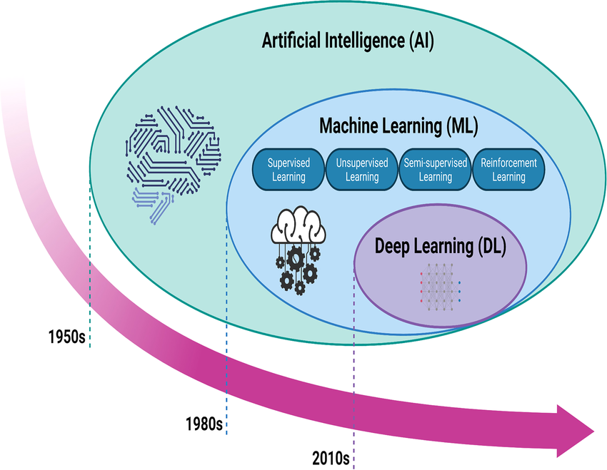

Artificial intelligence methods. Source: researchgate

The strong development of big data (Big Data) and the calculation ability has facilitated the method of machine learning and artificial intelligence (AI) to become an important tool in the volatility forecast. Different from traditional statistical models based on linear or defined distribution assumptions, these methods can be learned directly from data of nonlinear relationships, complex interactions, and hidden models that are hard to determine manually.

1. Linear regression

Linear regression is a platform technique in machine learning, modeling the linear relationship between dependent variables (here is the volatility) and a set of independent variables (such as past yields, technical indicators or macroeconomic factors). The model assumes that fluctuations at the present time can be forecasted by linear complexes of input characteristics.

Advantages:

– Easy to deploy and interpret: The regression coefficients provide clear information about the level of influence of each input variable.

– Light calculation: Suitable for limited resource systems and fast handling.

Limits:

– Assuming linear relationships: cannot grasp nonlinear relationships or interact between variables.Ineffective in a complicated financial environment and high fluctuations.

2. Decisive tree model: Random Forest and Xgboost

Random Forest: The Ensemble model uses many trees to train independence on sub -data sets (bootstrap samples). Each tree offers a forecast, the final result is synthesized by medium or voting. Random Forest has the ability to reduce the model variance and overcome overfitting phenomenon common in single trees.

XGBOOST (Extreme Gradient Boosting):  Is a powerful Boosting method to build a sequentially decisive tree, in which each new tree learns to fix the previous tree’s error. XGBOOST uses optimal techniques such as Regularization, Pruning, and Learning Rate to improve generalization and model performance.

Advantages: The ability to model nonlinear relationships and complicated interactions.Do not require standardization of input data.Can measure the importance of each variable.

Limits:Restricted interpretation due to complex and nonlinear model.Large training data and calculated resources are required, especially with XGBOOST.

For example, the results with the Garch model (1,1) of Bitcoin:

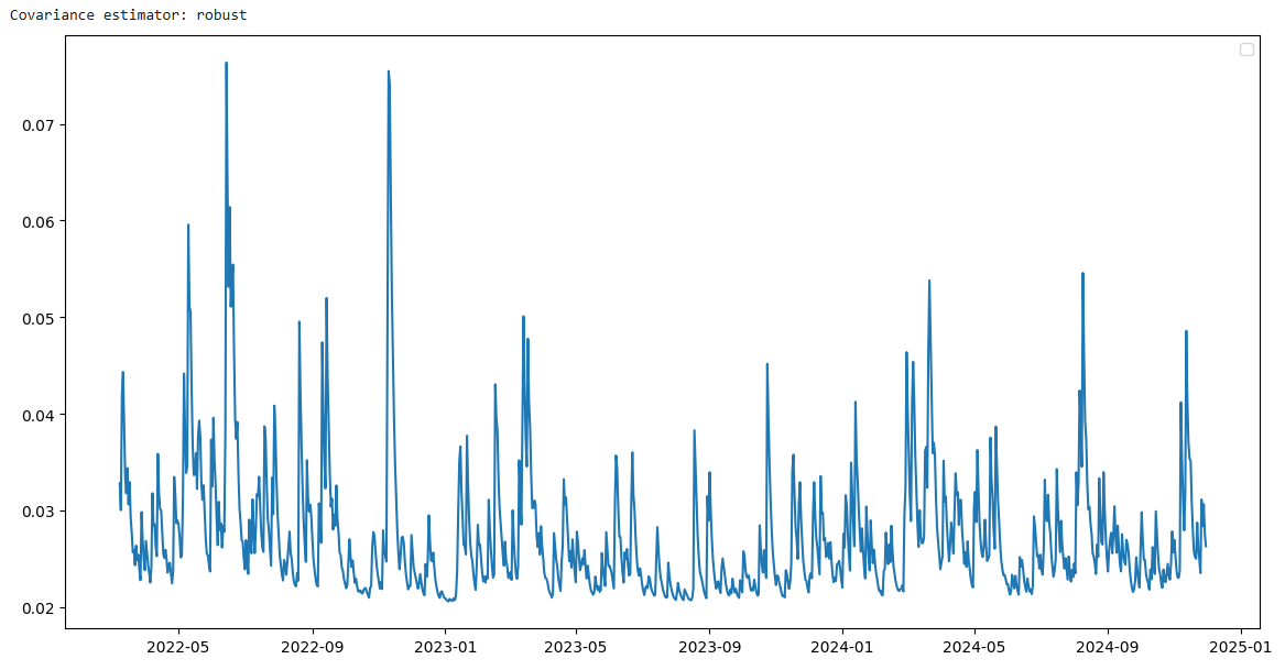
Conditional volatility is estimated from the Garch model (1,1) showing a clear fluctuating cluster phenomenon. The stages of strong fluctuations are often concentrated into clusters instead of random dispersion, reflecting the common characteristics of the financial market. The level of fluctuations changes over time, showing the appropriate garch model for risk modeling and volatility forecast.

Volatility Forecasting Methods: FAQ

1. What is volatility forecasting in crypto markets?
   Forecasting volatility means predicting future price swings of crypto assets (e.g. Bitcoin, Ethereum) by analyzing historical price data, on-chain metrics, order-book depth, and other indicators.
   
2. Which traditional statistical models are used?
   
   • GARCH (1,1): Captures volatility persistence and clustering with just three parameters.
     
   • ARCH: Models volatility clusters by linking today’s variance to past squared shocks.
     
   • ARIMA & EWMA: Use past returns and exponentially weighted moving averages for simple, fast estimates.
     
   • Rolling Variance: Computes standard deviation over a fixed window for an intuitive volatility gauge.
     
3. What are the strengths of traditional models?
   
   • Simplicity & Speed: Quick backtests on spot and derivatives (futures/options) markets.
     
   • Theoretical Rigor: Well-studied in finance literature and widely used in risk management.
     
4. Where do traditional methods fall short?
   
   • Struggle with black-swan events (e.g. DeFi hacks).
     
   • Miss nonlinear contagion between altcoins and stablecoins.
     
   • Fail to account for whale trades and on-chain spikes in funding rates.
     
   • Assume constant distribution of errors, ignoring leverage effects.
     
5. How do machine learning techniques improve forecasts?
   
   • Linear Regression: Quick baseline, interprets feature weights (e.g. technical indicators, macro data).
     
   • Random Forest & XGBoost: Model complex, nonlinear interactions among on-chain metrics, social sentiment, and technical signals without requiring data standardization.
     
6. What data inputs power AI-driven forecasts?
   
   • On-chain indicators: Active addresses, transaction volume, liquidity-pool flows.
     
   • Sentiment signals: Social volume, Google Trends, community chatter.
     
   • Options Implied Volatility: Skew and smile from crypto options markets.
     
   • Order-book depth: Bid/ask imbalance and funding-rate dynamics in perpetual futures.
     
7. When should I use hybrid approaches?
   Combine statistical models (e.g. GARCH) with machine learning (e.g. XGBoost) when facing volatile regime shifts—such as NFT mint rushes, protocol exploits, or major regulatory announcements—to capture both linear trends and complex nonlinear patterns.
   
8. How do I validate a volatility model?
   
   • Backtesting: Compare predicted vs. realized volatility on historical crypto price series.
     
   • Rolling-window evaluation: Measure forecast errors over different timeframes (e.g. 4-hour, daily, weekly).
     
   • Out-of-sample testing: Ensure robustness across bull, bear, and sideways crypto market cycles.
     
9. What’s the role of multi-timeframe analysis?
   Analyzing volatility indicators across multiple timeframes (e.g. 1-hour, 4-hour, daily) helps confirm clustering patterns and reduces false signals by aligning short-term spikes with longer-term trends.
   
10. How do I choose the right volatility forecasting method?
    
    • Data availability: Use Rolling Variance or EWMA for limited data; opt for GARCH or ARCH with longer histories.
      
    • Computational resources: Leverage machine learning if you have GPU/CPU capacity; otherwise, stick with fast traditional models.
      
    • Forecast horizon: For intraday estimates, combine high-frequency on-chain signals with EWMA; for longer horizons, GARCH or XGBoost may offer better performance.

Conclusion

Volatility is forecasted to be a continuous development field, playing a central role in modern finance. Statistical models such as Garch are still a solid foundation thanks to the interpretation and efficiency, while the methods of machine learning and AI opens up the outstanding potential in complex data exploitation. Choosing the right model requires careful consideration between data, forecasting, and available resources. With a flexible combination and strict assessment, these methods will continue to play an important role in shaping smart and sustainable financial decisions.